913
Technical Committee 104 /
Comité technique 104
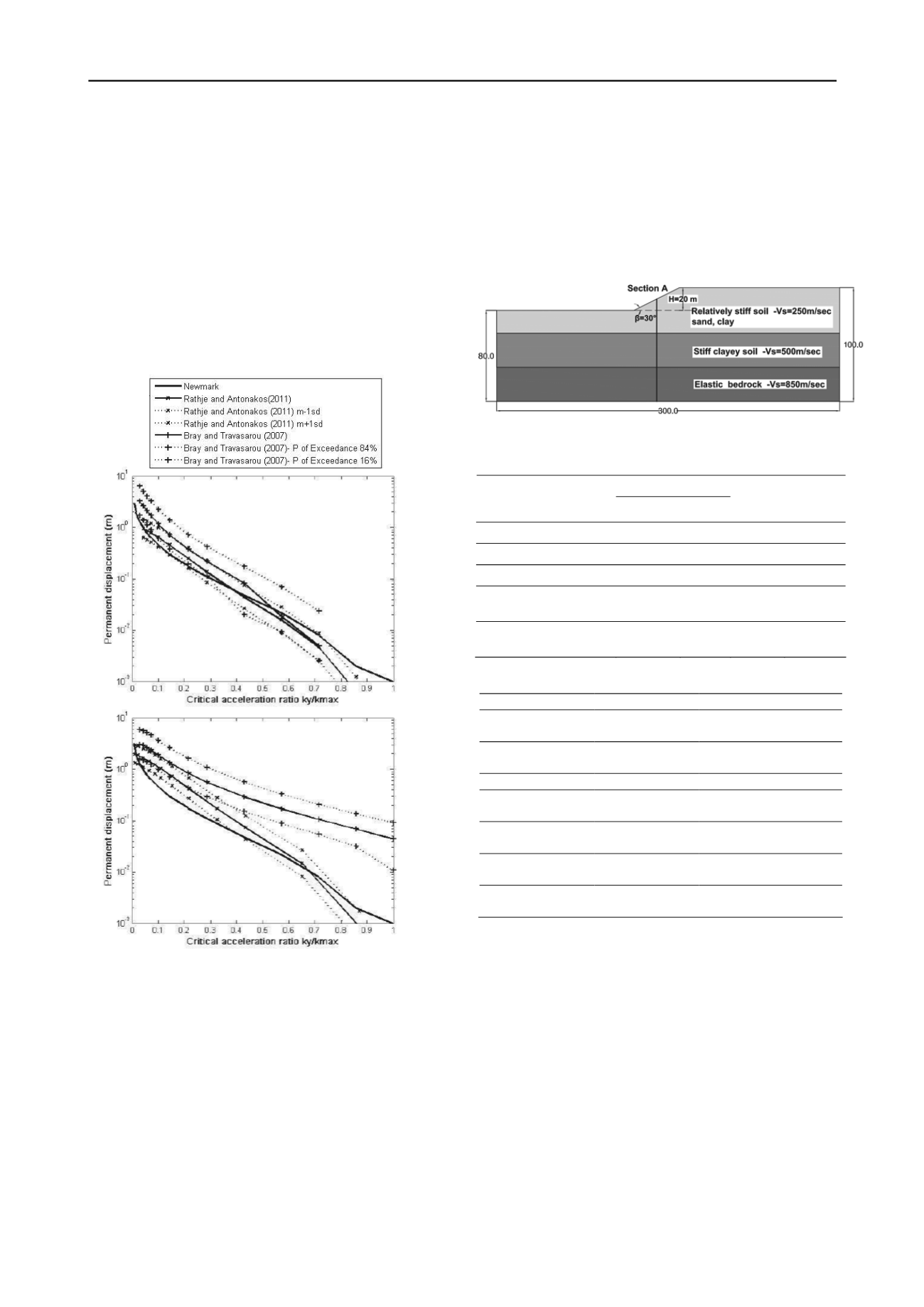
acceleration ratio, whereas in Rathje and Antonakos (see Fig.
2b) this trend does not seem to be influenced by the critical
acceleration ratio. Contrary to the previous models it seems that
the importance of the frequency content is not taken into
account in the Bray and Travasarou coupled model, which
predicts slightly larger displacements for the higher frequency
input motion (see Fig. 2c). The latter model generally predicts
larger displacements compared to Newmark rigid block and
Rathje and Antonakos decoupled models. In particular, the
difference in the displacement prediction is by far more
noticeable for the flexible (Fig. 3b) compared to the nearly rigid
(Fig. 3a) sliding mass. Displacements computed using Rathje
and Antonakos predictive equations are closer to the Newmark
rigid block model. The comparison is even better for the higher
frequency input motion and for the lower level of shaking.
The
Figure 3. Comparison of the different Newmark-type models when
considering a nearly rigid (a) and a relatively flexible (b) sliding mass
for a certain earthquake scenario (Pacoima scaled at 0.7g)
3 COMPARISON WITH THE DYNAMIC NUMERICAL
ANALYSIS
The second goal is to compare the Newmark-type analytical
models with an a-priori more accurate numerical model. For this
purpose a two- dimensional fully non-linear FLAC (Itasca,
2008) model has been used. The computed permanent
horizontal displacements within the sliding mass for the two
idealized step-like slopes, characterized by different flexibility
of the potential sliding surface, are compared with the three
Newmark-type models.
The geometry of the finite slope is shown in Figure 4. The
discretization allows for a maximum frequency of at least 10Hz
to propagate through the grid without distortion. Free field
absorbing boundaries are applied along the lateral boundaries
whereas quiet boundaries are applied along the bottom of the
dynamic model to minimize the effect of artificially reflected
waves. The soil materials are modeled using an elastoplastic
constitutive model with the Mohr-Coulomb failure criterion,
assuming a non-associated flow rule for shear failure. Two
different soil types are selected for the surface deposits to
represent relatively stiff frictional and cohesive materials. The
mechanical properties for the soil materials and the elastic
bedrock are presented in Table 2.
Figure 4. Slope configuration used for the numerical modeling
Table 2. Soil properties of the analyzed slopes
Relatively stiff soil
Parameter
sand clay
Stiff
soil
Elastic
bedrock
Dry density (kg/m
3
)
1800
1800
2000
2300
Poisson's ratio
0.3
0.3
0.3
0.3
Cohesion c (KPa)
0
10
50
-
Friction angle φ
(degrees)
36
25.0
27
-
Shear wave
Velocity V
s
(m/sec)
250
250
500
850
Table 3. Selected outcropping records used for the dynamic analyses
Earthquake
Record station
Mw
R(km) PGA(g)
Valnerina, Italy
1979
Cascia
5.9
5.0
0.15
Parnitha, Athens
1999
Kypseli
6.0
10.0
0.12
Montenegro 1979
Hercegnovi Novi
6.9
60.0
0.26
Northridge,
California 1994
Pacoima Dam
6.7
19.3
0.41
Campano Lucano,
Italy 1980
Sturno
7.2
32.0
0.32
Duzce, Turkey
1999
Mudurno_000
7.2
33.8
0.12
Loma Prieta,
California 1989
Gilroy1
6.9
28.6
0.44
The initial fundamental period of the sliding mass (T
s
) is
estimated using the simplified expression: T
s
= 4H/V
s
, where H
is the depth and V
s
is the shear wave velocity of the potential
sliding mass. The depth of the sliding surface is evaluated equal
to 2m for the sandy slope and 10m for the clayey one by means
of limit equilibrium pseudostatic analyses. The horizontal yield
coefficient, k
y
, is computed via pseudostatic slope stability
analysis equal to 0.16 and 0.15 for the 30
o
inclined sand and
clayey slopes respectively.
The seismic input applied along the base of the dynamic
model consists of a set of 7 real acceleration time histories
recorded on rock outcrop (see Table 3) and scaled at PGA=0.7g.
To derive the appropriate inputs for the Newmark-type methods
that include the effect of soil conditions, and to allow a direct
comparison with the numerical results, we computed the time
histories at the depth of the sliding surfaces through a 1D non-
linear site response analysis considering the same soil properties
as in the 2D dynamic analysis. It is noticed that the 1D soil
profile is located at the section that approximately corresponds
(a)
(b)


